
DCNv3: Unlocking Extremely High-Order Feature Interactions with Exponential Cross Layers
DCNv3 allows modeling feature interactions of degrees unseen before in the DCN family of architectures - and has quietly taken over the Criteo leaderboard


The Deep and Cross family of neural architectures is one of the most successful solutions for click-through rate prediction problems, as evidenced by its consistent place in the top of ML leaderboards such as the Criteo display ads benchmark dataset.
First introduced by Google in 2017 (Wang et al 2017), the key idea is to generate all possible feature “crosses” in a brute-force manner, which was a significant breakthrough in recommender systems and replaced the previous practice of tediously engineering cross features by hand, popularized by Google’s Wide&Deep architecture (Cheng et al 2016).
The crux of DCN is that the more cross layers we stack, the higher the order of feature interactions we can model. One layer results in second-order interactions (features with features), two layers result in third-order interactions (features with features with features) and so on. In theory, this should allow us to make our model extremely capable simply by adding more cross layers. In practice though, researchers soon found that DCN’s performance saturates after just 2-3 layers, which was a disappointing result.
The reason for DCN’s failure to scale were two-fold:
DCN’s interactions were vector-wise (i.e., using the dot product), not bitwise (i.e, using the element-wise product), and
As we stack more cross layers, we introduce not only more signal into the model but also disproportionately more “cross noise” from entirely meaningless feature crosses, increasing the risk of overfitting.
The first of these two limitations was addressed in DCNv2 (Wang et al 2020), again from Google, which was the first DCN-like model modeling bit-wise feature interaction. Combined with several other innovations such as Mixtures of Experts and LoRA, the authors were able to stack 4-5 cross layers and still see improvements in model performance. This observation proved that the higher expressiveness of bitwise interactions is indeed useful for DCN-like models.
The second of DCN’s limitations, cross noise, was addressed by a group from Fudan University, China, and Microsoft Research. The paper “Towards Deeper, Lighter and Interpretable Cross Network for CTR Prediction” (Wang et al 2023) introduced GDCN, short for Gated DCN, which is essentially a variant of DCNv2 with the addition of a gating network, which learns a scalar weight for each feature cross. Interestingly, as we train the model, the gating network learns to suppress noisy crosses (the weight will be near 0), while up-weighing informative crosses (the weight will be near 1).
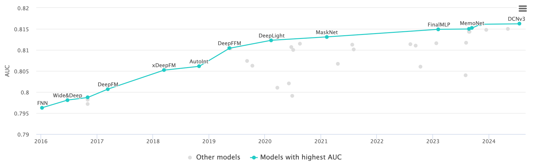
Ever since its introduction in November 2023, GDCN has been leading the Criteo benchmark. This changed in the summer of 2024 with the introduction of DCNv3, work done by Anhui University, China, and Huawei (Li et al 2024). DCNv3 once again introduced several improvements that made the DCN architecture more capable than ever before, most importantly via the introduction of its novel exponential feature crossing method. Let’s take a look.
Exponential crossing

The main innovation in DCNv3 is the addition of the Exponential Cross Network (ECN), which allows the model to produce higher-order feature interactions far more efficiently than traditional Linear Cross Network (LCN).
As a reminder, linear crossing in DCN-like models works by recursively combining features layer by layer, where each layer produces interactions of a higher order. For example:
Layer 1 produces second-order interactions (features with features),
Layer 2 produces third-order interactions (features with features with features),
Layer 3 produces fourth-order interactions, and so on.
The recursive formula for LCN is:
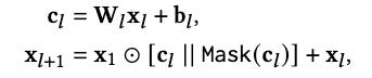
where c_l is a linear projection of the input, and x_{l+1} computes the interactions of with the original feature vector, x_1 using the element-wise product, hence incrementing the interaction order by 1 for each added layer. (“Mask” is DCNv3’s self-masking operator which we’ll introduce in a bit.)
Note that we also add the inputs x_l themselves back to the outputs. Technically, this is a skip connection, similar to those found in a ResNet architecture. In this particular case, the addition of skip connections enables a hierarchy of feature interactions by ensuring that each layer's output not only includes the higher-order interactions generated in that layer but also retains the lower-order interactions from all preceding layers.
ECN takes this one step further by allowing interactions to grow exponentially with each layer, that is,
Layer 1 produces second-order interactions,
Layer 2 produces 4th-order interactions,
Layer 3 produces 8th-order interactions,
and so on. Its recursive formula is:

which is identical to LCN with the key difference that we cross the crosses with themselves, not with the original feature vector (x_1), allowing for faster growth — doubling the interaction order with each additional layer instead of just incrementing them by 1. The exponential indexing may be a bit confusing at first, but it is really just a formality to ensure that the layer index stays proportional to the feature interaction order.
The DCNv3 architecture is then simply a fusion of LCN and ECN modules using the Mean operation,

where y_D and y_S are the sigmoid-activated output from the LCN and ECN, respectively, W and b are learnable weights and biases, and y is the final prediction obtained by averaging.
Self-masking
Another innovation in DCNv3 is the Self-Mask operation, which is designed to address the problem of cross noise. In contrast to GDCN, the mask in DCNv3 is not learned, but instead derived directly from the activation logits inside a cross layer. In particular, the mask value for a logit is simply the layer-normalized logit clipped at 0 (i.e., setting all negative values to 0). The motivation behind this design is to ignore negatively activated neurons in these cross layers, which the authors claim constitute cross noise.
Formally, we can write the self-mask operation as

where LN is the layer-norm operator.
Note that this form is similar but not identical to ReLU: like ReLU, we clip the negative values to 0, but unlike ReLU we use these clipped values as a multiplier, not as the output directly, hence preserving the information contained in the original (unnormalized) logits.
Tri-BCE loss
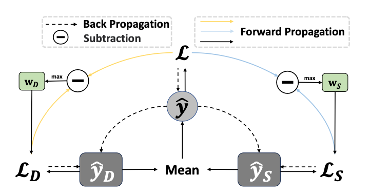
In order to ensure that both sub-networks (DCN and ECN) both learn equally during training, and one is not favored over the other, DCNv3 adds the losses for LCN and ECN themselves as auxiliary losses back into the total loss. The authors call this combined loss the “Tri-BCE” loss. We can write it as

where w_S and w_D are dynamic weights that are learned during training. Using an ablation experiment, the authors estimate that the addition of Tri-BCE loss accounts for around 0.5% Train AUC gain on Criteo, so indeed it does appear to play an important role in training DCNv3.
Experimental result

The authors did an extensive suite of experiments, where they compared the predictive performance of DCNv3 with 15 competing algorithms on a suite of 6 benchmark datasets, and find that DCNv3 beats all competitors on all of these datasets. For example, on the Criteo display ads dataset, they beat DCNv2 by 0.17% AUC, and the closest competitor, FINAL (Zhu et al 2023), by 0.13% AUC. (Like DCNv3, FINAL grows feature interactions exponentially, but unlike DCNv3, it does so using implicit interactions built with non-linear attention layers instead of explicit interactions built with cross layers.)
DCNv3 works best with just the right number of cross layers to avoid either under-fitting (too few layers) or over-fitting (too many layers), and curiously that number appears to depend on the dataset. The authors give 2 examples,
for Criteo, the best-performing DCNv3 model has 4 layers, corresponding to feature interactions of 16th order,
for KDD12, the best-performing DCNv3 model has 6 layers, corresponding to feature interactions of 64th (!) order.
Note that in order to be able to model feature interactions of the 64th order in a standard DCN model, one would need to stack 64 layers, not 6, resulting in ~10X the number of model parameters. This illustrates the major advantage of DCNv3, that is, being able to model extremely high-order feature interactions (which appear to be necessary for at least some datasets) with relatively few model parameters.
My take
DCNv3 represents a significant leap forward in the evolution of the Deep and Cross architecture, making it (perhaps for the first time) computationally feasible to model extremely high-order feature interactions.
One weak spot in this work is certainly the self-masking heuristic of simply clipping based on the normalized logits — the authors themselves appear to acknowledge this by commenting that “Other mask mechanisms can also be used here”. I would expect better performance when we let the model learn itself which crosses to pay attention to and which to ignore, either using self-attention, such as done in AutoInt (Song et al 2018), or using gating, such as done in GDCN (Wang et al 2023). Curiously, the authors did compare against neither of these in the paper, but based on paperswithcode the improvement of DCNv3 over GDCN is a mere 0.01% AUC on Criteo.
It is a surprising finding that there are problems that require an extremely high degree of feature interactions as enabled by DCNv3, such as 64th order in the KDD12 dataset. It would be interesting to investigate further what exactly these 64th-order interactions mean, and whether they truly indicate a new signal that cannot be mined from lower orders, or simply replicate existing signal already seen in the lower orders.
Lastly, the modular nature of DCNv3, combining both linear and exponential crossing, opens the door for further innovations. Future research could explore dynamic mechanisms to adaptively balance the two types of crossing based on the dataset, borrowing from Mixture of Experts approaches. It would also be interesting to combine DCNv3 with dynamic computation. As we’ve seen, not all problems are alike: certain problems appear to require modeling of higher-order feature interactions, and others not. Ultimately, then, a model architecture that could dynamically adapt to the data present, similar to Google’s MoD architecture (Raposo et al 2024), could turn out to be a capable and efficient all-purpose modeling architecture.