Towards a Scaling Law for Recommender Systems

Meet Wukong - a surprisingly simple yet effective architecture revolutionizing ranking models once again

In Chinese culture, Sun Wukong is a rebellious and powerful mythological monkey with superhuman strength, speed, and shape-shifting abilities.

Feature interactions are one of the most important components in recommender systems. Lots of the research of the past decade went into how to best generate these feature “crosses”, and how to best use them in the model.

One of the first pieces of work demonstrating the effectiveness of feature crosses was Google’s 2016 “Wide & Deep”, in which the authors hand-engineered cross features for the Google Play store such as

AND(installed_app='netflix', candidate_app='hulu')

which is 1 if the user has Netflix installed and the candidate app to be ranked is Hulu. By adding a large number of such crosses to their neural network model, the authors were able to get 1% gains in app conversions.

The game changed considerably with the introduction of FMs, or Factorization Machines (Guo et al 2017), which generate feature crosses exhaustively simply by taking dot products between feature embeddings of all possible feature combinations,

FM(X) = XXT,

where X is the (n x d)-dimensional feature matrix, with n the number of features and d the embedding dimension.

The success of FMs spawned new advancements such as DCNv2 (Wang et al 2020), which uses element-wise instead of vector-wise multiplication for even more fine-grained feature crosses. DCNv3, its 2024 successor, is currently still leading the Criteo Display Ads competition.

Alas, one (important) question remained unanswered: do these models have a scaling law? Meaning: does model performance increase as we increase parameter count?

No, argue the authors of the recent paper “Wukong: Towards a Scaling Law for Large-Scale Recommendation” (Zhang et al 2024). The existing models are not enough, so the argument, because they fail to scale to bigger datasets, or, for that matter, to any dataset of any size (smaller or larger). Instead, we need to rethink the design of the interaction layer and make it more dynamic and scalable to any problem size.

Meet Wukong, a new take on the FM design with clever optimization tricks designed to do just that.

The Wukong layer

Left: a Transformer block, the building block for scalable LLMs. Right: a Wukong block, presumably the building block for scalable Recommenders.

A single Wukong layer transforms a set of input embeddings (X_i), each generated using an embedding table, into a set of output embeddings (X_i+1) as

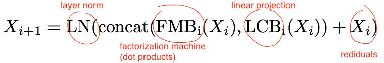
where

• LN is layer normalization,

• FMB (“factorization machine block”) creates feature crosses using dot products between the rows in X_i,

• LCB (“linear compression block”) adds a compressed representation of the original inputs back into the outputs such as to increase the breath of cross orders (the second layer, for example, will not only create crosses of crosses but also crosses of crosses and the original features, i.e. both 4th and 3rd order interactions),

• the last term is a residual connection to improve information flow of gradients as we stack more layers.

Formally, the two main components of the model are

FMB(X) = MLP(LN(flatten(FM(X)))),
LCB(X) = WX,

where FM is Wukong’s “optimized FM” (which we’ll discuss below) and W is a learnable projection matrix of dimension (n x k_LCB).

And that’s it! The Wukong layer really is remarkably simple.

Binary exponentiation

Importantly, as we stack more Wukong layers, feature interactions grow exponentially because each subsequent layer creates all cross from all of its input features, including the crosses themselves — the authors call this “binary exponentiation”:

• the first layer outputs second-order interactions (features with features) as well as first-order interactions (the features themselves),

• the third layer outputs 4th, 3rd, 2nd, and first order interactions,

• the fourth layer outputs all interactions from 8th down to first order,

and so on. Similar to DCNv3, this exponential growth gives the model the advantage of being able to capture higher-order feature interactions with fewer layers and hence fewer parameters compared to models with linear order growth, such as DCNv2.

Dimensionality preservation via Optimized FM

Naively computing XX^T in each subsequent Wukong layer would be a bad idea. Consider a simplified example with just n=4 input embeddings. Then,

• the output of the first layer would be a 16-dimensional matrix, containing one dot product per feature pair,

• the output of the second layer would be a 256-dimensional matrix,

• the output of the third layer would be a 65,536-dimensional matrix,

and so on. Doing this would blow up our memory. Instead, similar to DCNv2, Wukong uses low-rank projection to shrink the interaction matrix from

FM(X) = XXT [n,n]

(where n is the number of features) to

FM(X) = XXTY [n,kFMB]

where Y is a learnable projection matrix of dimension (n x k_FMB). The authors call this version “optimized FM”.

This simple projection trick allows for dimensionality preservation, that is, the output of a Wukong layer has the same dimension as its input, as long as

kFMB + kLCB = n.

(Adding the residuals in the Wukong equation is only possible thanks to this dimensionality preservation trick.)

Empirical results

The authors show that Wukong beats 7 competing model architectures on a suite of 6 benchmark datasets. For example, on the KuaiVideo dataset (video recommendation), Wukong beats its closest competitors, FinalMLP and MaskNet, by around 0.4% AUC, and DCNv2 by more 0.54% AUC.

On company-internal data, the authors once again prove that Wukong works best, but also demonstrate its superior scaling law: as we increase the number of model parameters (i.e., stack more Wukong layers), model performance improves, while other models seem to plateau at a size of around 600B parameters.

Empirically, Wukong’s scaling law relationship between model size and performance is

y = −100 + 99.56x0.00071.

0.00071 may seem like a small number but what matters really is that it is non-zero: this means that “all” we need to make better predictions are more GPUs.

Coda

There are multiple things that I find worth highlighting in this work.

First, ever since DCNv2 the consensus in the domain has been that bit-wise interactions work better than vector-wise ones because they are more expressive. Wukong reverts this conclusion once again, showing that in fact dot products are really you need. This is one of those rare “Attention is all you need” moments where making something simpler actually results in better performance.

Second, the scaling law exponent is really, really small. Compared to LLMs, around 100-1000 times smaller. This is a great datapoint showing just how much harder recommendation problems — with their vast and ever-changing vocabularies — are compared to language problems. This also means that, unless we find an architectural design with a more favorable exponent, something like a “ChatGPT moment” for recommenders is still very far into the future.

And third, because of the small exponent, the fact that the authors weren’t able to measure the end of the scaling law in their own experiments. In the authors’ own words,

Understanding the exact limit of Wukong’s scalability is an important area of research. Due to the massive compute requirement, we have not been able to reach a level of complexity where the limit applies.

How good can recommendations get? At the moment, no one knows. Which makes recommender systems such an exciting place to work in.

Until next time!

More on the topic

• The Rise of Deep and Cross Networks in Recommender Systems

• DCNv3: Unlocking Extremely High-Order Feature Interactions with Exponential Cross Layers

• A Tour of the Recommender System Model Zoo (Part II)

• A Tour of the Recommender System Model Zoo (Part I)