A Friendly Introduction to Large Language Models (LLMs)

A comprehensive primer on tokenization, embedding generation, multi-headed self-attention, causal masking, Transformer blocks, model variants, and training paradigms

Large Language Models (LLMs) are one of the most scientifically interesting and practically useful Machine Learning applications in the industry today. To newcomers, much of the scientific jargon like “attention”, “tokenization”, or “Transformer block” may appear intimidating, however these concepts are really not as complicated as they may first seem.

At a high level, a modern LLM is simply a stack of many Transformer blocks, each containing self-attention layers that learn the relationships between words in input sequences from human language. With enough data and a number of clever modeling tricks invented over the years, the model will eventually be able to produce human-like text on its own.

In this primer, we’ll break down the fundamental building blocks of a Transformer-based LLM, including:

• tokenization and embeddings,

• multi-headed causal self-attention,

• the ingredients of the Transformer block,

• Transformer model variants, and

• training paradigms for Transformer-based LLMs.

Happy learning!

Tokenization and embeddings

A single word is being transformed into an embedding sequence

Neural networks learn from numeric data, so any discussion of LLMs needs to start with how we transform sequences of unstructured text into numbers. There are 3 steps: (1) tokenization, (2) token embeddings, and (3) positional embeddings.

Tokenization is an algorithm that chunks up a sentence into a sequence of sub-word tokens of fixed cardinality, making the problem more tractable compared to simply treating each new word as a new feature: tokenization is robust against the introduction of new words, typos, foreign words, and so on. No matter the input, it can be deterministically mapped into a set of pre-determined tokens from the model’s vocabulary (i.e. its set of tokens).

Tokenization algorithms, such as Byte Pair Encoding (BPE), WordPiece, or SentencePiece, first chunk up words into characters, and then iteratively merge these characters into the most common combinations observed in the data. For example, the word “unaffordable” may be first segmented into the sequence ["u", "n", "a", "f", "f", "o", "r", "d", "a", "b", "l", "e"], and eventually be merged into the sequence ["un", "afford", "able"], resulting in 3 tokens.

The size of the vocabulary can vary depending on several factors, including the corpus used for training, the specific requirements of the task, and the granularity desired by the developers of a particular model. For example, OpenAI’s GPT-2 uses BPE with a vocabulary of around 50K tokens, while Google’s BERT uses WordPiece with a vocabulary of around 30K tokens. Ultimately, the choice of the vocabulary size represents a tradeoff between computational efficiency and granularity: a model with a larger vocabulary will be able to model language at a more granular level, but it will have larger embedding tables requiring more FLOPs as well as more memory.

Token embedding layers are linear layers that map each token in the input sequence into a low-dimensional, dense vector: the input dimension of this layer is the size of the vocabulary, and the output dimension is the embedding dimension. It has been found that larger embedding sizes usually work better, perhaps a reflection of the high information density contained in human language: for example, the largest variants in the GPT series have embedding dimensions of 768! The embedding layer is randomly initialized, and learnt during training.

At inference time, we can treat this layer as a look-up table, that is, given an input token we can simply retrieve its embedding directly from the stored weights in the embedding layer.

Positional embedding layers learn the information contained in the order of the tokens in the input sequences. A naive way would be to pass the position itself into the model (0,1,2,3,…), however these ordinals would not be a good signal for a neural network to learn from: they’re hard to combine with the token embeddings, and the model may easily overfit to the ordinal itself. A better way is to represent these positions as embeddings themselves.

One of the most common positional embedding algorithms is sinusoidal embedding, introduces in the pivotal paper “Attention is all you need” (Vaswani et al 2017), defined as follows:

where pos is the position in the sequence, i is the dimension index, and d is the total number of dimensions. For example, in the simplified case of just 4 dimensions, the positional embeddings would be:

position 0: [0,1,0,1]
​position 1: [0.8415,0.5403,0.0100,0.99995]
​position 2: [0.9093,−0.4161,0.0200,0.99980]
position 3: [0.1411,−0.9900,0.0300,0.99955]
position 4: [−0.7568,−0.6536,0.0400,0.99920]
​position 5: [−0.9589,0.2837,0.0500,0.99875]

and so on, depending on the length on the sequence. The advantage of this approach is that it is parameter-free, which means fewer parameters that need to be learnt and less compute. Another advantage is that it generalizes to sequence lengths unseen during training. Vaswani et al also compared this approach with learned positional embeddings (similar to learned token embeddings), and found no performance gains from doing so.

As a final step, we simply sum the token embeddings and positional embeddings, so that the resulting sequence of embedding vectors contains both pieces of information which can then be modeled in the attention layers.

Self-attention

Multi-headed attention block (source: Attention is all you need)

At a high level, self-attention layers transform input sequence into output sequences in a contextual way, that is, the output at a particular position does not only depend on the information in that position itself, but also on the relationship with all the other information in all the other positions, i.e., on its context.

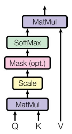
Under the hood, self-attention performs the following 3 steps:

1. Projection: we project the input sequence X into 3 new sequences named K (keys), Q (queries), and V (values), using 3 learnable projection matrices.

2. Attention scoring: we compute the dot products between key vectors and query vectors, and normalize these dot products using a softmax. We call these normalized dot products the attention scores. They tell us how much these two token positions "attend to each other”, i.e. when looking at the key token, how relevant is the query token in understanding its meaning?

3. Weighting: we weigh each value token by the corresponding attention value computed in step 2.

In (PyTorch) code:

import torch
import torch.nn as nn
import torch.nn.functional as F

class SimpleSelfAttention(nn.Module):
    def __init__(self, embed_size):
        super(SimpleSelfAttention, self).__init__()
        self.embed_size = embed_size
        self.values = nn.Linear(embed_size, embed_size, bias=False)
        self.keys = nn.Linear(embed_size, embed_size, bias=False)
        self.queries = nn.Linear(embed_size, embed_size, bias=False)
        self.fc_out = nn.Linear(embed_size, embed_size)

    def forward(self, values, keys, query, mask=None):
        # Apply the linear transformations
        values = self.values(values)
        keys = self.keys(keys)
        queries = self.queries(query)

        # Compute the dot products between queries and keys
        energy = torch.matmul(queries, keys.transpose(-2, -1))
        energy /= (self.embed_size ** 0.5)

        # Causal masking
        if mask is not None:
            energy = energy.masked_fill(mask == 0, float("-1e20"))

        # Attention (Softmax normalization of energies)
        attention = torch.softmax(energy, dim=-1)

        # Multiply attention weights by the values
        out = torch.matmul(attention, values)

        # Pass through a final linear transformation
        out = self.fc_out(out)
        return out

Note that here we also normalized the attention scores by the square root of the embedding dimension. The purpose of this normalization is to make the model robust against changes in the embedding dimension — the magnitude of two high-dimensional vectors tends to be large simply due to their dimensionality. Vaswani et al tested this scaling factor and observed that it resulted in better training stability and model performance compared to not scaling or using other scaling factors.

Causal masking

In the code above you’ve noticed an optional mask argument in the forward pass: this can be used to introduce the causal mask, which is a critical component in models used for generating text responses to user prompts.

The key idea behind causal masking is that we want to prevent the model from using future information: each token should only attend to tokens preceding it, not to tokens that come after it. In practice, we do this by passing as mask argument a matrix with ones on the lower triangle and ones on the upper triangle:

# causal mask with sequence length 5

1, 0, 0, 0, 0,
1, 1, 0, 0, 0,
1, 1, 1, 0, 0,
1, 1, 1, 1, 0,
1, 1, 1, 1, 1

By replacing the masked attention scores with a very large negative value (here: -1e20) before the softmax computation, effectively we zero these scores out.

Multi-headed attention

Multi-headed attention block (source: Attention is all you need)

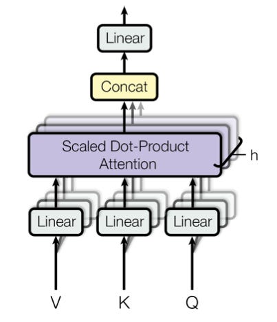
Multi-headed attention simply means that instead of having just a single attention module we add multiple attention modules, each generating their own K, Q, V projections, attention scores, and attention-weighted outputs. We then combine all of these output sequences by first concatenating them and then passing this concatenated vector through a final projection matrix, the “output” matrix O.

In practice, many heads work much better than a single head because they allow the model to learn grammatical relationships, semantic relationships, long-range dependencies, co-references, sentiment, punctuation, and more, all at the same time. The more heads we add, the more nuanced the contextual information that can be learned together, resulting in superior performance. For example, BERT-Base, GPT-1, and GPT-2 are all models with 12 heads, but newer models usually have more: the largest GPT-3 variant has 96 heads, and the largest T5 variant has 128 heads!

A common modeling trick is to reshape the dimensionality of the embeddings from d to d/H x H, where H is the number of attention heads, such as to preserve the total number of parameters in the model. In this case, when introducing more heads, it is important that the embedding dimension is large enough to support the extra heads.

LayerNorm

LayerNorm is an algorithm that normalizes the outputs by subtracting the mean and dividing by the standard devision taken over the embedding dimension. This normalization guarantees that activations stay within the range (-1,1) even when stacking a large number of layers, which has been found to improve training stability.

We use LayerNorm instead of BatchNorm (where we’d normalize over the batch dimension instead of the embedding dimension) because the latter assumes that batch sizes are always the same, including at inference time, which is usually not the case in LLMs: in the extreme case an inference request may consist of just a single input sequence.

Feed-forward module

So far, every transformation in the model has been linear: the multi-headed self attention module is computing linear matrix multiplications, and the LayerNorm module is simply normalizing these outputs. The feed-forward module serves the important purpose of adding non-linearity to the model, allowing it to learn more complex patterns from the data.

The FFN module in a Transformer consists of 2 linear layers with a non-linear activation in between, where the hidden dimension is usually 4x larger than the embedding dimension. Commonly used non-linear activations are ReLU (BERT), GeLU (GPT series), SwiGlu (Llama-2), and GeGLU (Gemma). In the paper “GLU Variants Improve Transformer”, Noam Shazeer showed that (as the title implies) these GLU variants are particularly effective activation functions in Transformer models.

Note that the FFN module is also oftentimes called a "pointwise" transformation, which simply refers to the fact that we process each token individually, irrespective of its surroundings. In contrast, the attention module is performing global processing of its input, that is, looking at the input sequence holistically.

Putting it all together: the Transformer architecture

The Decoder-only Transformer architecture. Image by Cameron Wolfe

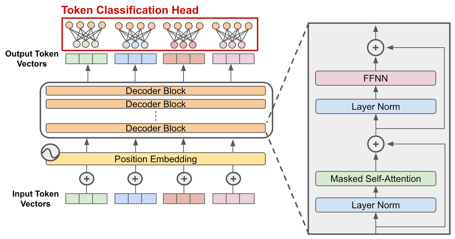
We now have all the ingredients together to build a Transformer block, the fundamental building block of modern LLMs. The Transformer block is simply a sequence of:

1. LayerNorm

2. Multi-headed self-attention

3. Another LayerNorm

4. Feed-forward module

One additional detail is the introduction of skip connections that bypass the attention module and the FFN module, i.e. we take the inputs to these modules and add them back to their outputs. Skip connections, first introduced in the ResNet architecture used in Computer Vision, prevent gradients from becoming too small as we stack more layers, a problem known as the vanishing gradient problem.

A Transformer model is simply a stack of many such Transformer blocks transforming input sequences into output sequences. For example, the largest Llama-2 variant stacks 40 Transformer blocks, while the largest variants in the GPT series stack 96 Transformer blocks!

Lastly, in order to make predictions, we add a final module, the classification task head. This head takes as input the transformed sequence and outputs a prediction, such as the prediction for the next word in the sequence, the sentiment score of the input sequence, or something else, depending on the application.

The 3 Transformer variants

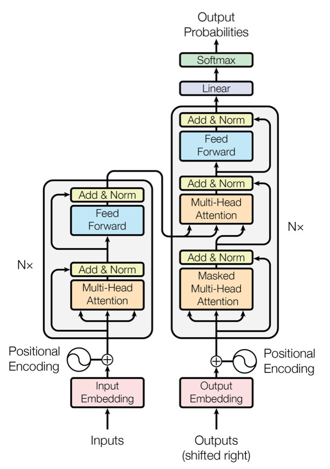
The particular type of Transformer architecture we’ve seen above is known the Decoder-only Transformer, and it the backbone of models such as GPT, Llama, Gemma, etc. However, this type is different from the original Transformer architecture proposed in Vaswani et al’s 2017 “Attention is al you need” paper.

In the 2017 work, the authors added a second tower, the encoder tower, with its own Transformer blocks, and feed the outputs of the encoder into a second attention module in the decoder block. The main difference between the encoder and the decoder is that the encoder does not use causal masking, instead looking at the entire input sequence at once.

The encoder-decoder Transformer contains an encoder tower for input sequences and a decoder tower for output sequences

Unlike the decoder-only Transformer, which outputs a prediction given an input sequence, the encoder-decoder Transformer is a sequence-to-sequence model: it learns to map one sequence into another sequence. This is useful for translation tasks, where we want to translate user prompts from one language into another language, but not so useful for text generation tasks, where all we want to is produce a response given a prompt.

Lastly, there’s a third variant, namely the encoder-only model, which drops the decoder tower instead of the encoder tower, BERT being the most famous example. Encoder-only transformers don’t have causal masks, and are therefore not that useful for generating text. Instead, they are used for particular downstream applications that require modeling the entire text sequence at once such as sentiment classification, named entity recognition, or question answering.

Training Transformer models

Transformer models are usually trained using 2 or 3 stages, depending on the application:

1. Unsupervised pre-training: during this stage, we train the model on a large corpus of text data such as Wikipedia or News articles. Unsupervised means that we don’t provide any labels, just the data itself, and train the model by letting it predict the next token in the sequence (autoregressive training) or masked tokens within the sequence (masked language modeling).

2. Supervised fine-tuning: during this stage, we give the model specific, human-curated pairs of text prompts and labels to learn from, such as question-answer pairs, text blurbs with the corresponding sentiment, etc. It has been found that during this fine-tuning stage just the last few layers of the model change, which indicates that after pre-training the early layers contain statistical information about generic, task-agnostic linguistic patterns that don’t need to change for different downstream tasks.

3. Reinforcement learning with human feedback (RLHF): during this stage, human AI trainers give the model prompts and rank its responses. That rank is then used as a reward in a reinforcement learning algorithm. RLHF, pioneered in InstructGPT, is an extremely effective way to improve conversational coherence of the model because it learns directly from human feedback based what it just did, as opposed to just learning to predict labels on historic data (which can be easily memorized with enough parameters).

Each of these stages has its own challenges and technical complexities that I won’t go into detail here. However, one common theme that you’ll find in the literature is that companies will usually reveal very little about their training data when releasing a new model. This is on purpose: while the architecture behind modern LLMs has converged largely to the Transformer architecture (with only subtle variations), the competitive advantage of one model over another really comes from superior training data and processes.

Summary and outlook

To summarize, LLMs first transform human language into sequences of dense embeddings using tokenization, learned embedding tables, and (fixed) positional embeddings, and then pass these sequences through a number of Transformer blocks, each of which contains multi-headed, causal self-attention modules (for leaning relationships between tokens) and feed-forward layers (for generating non-linear signals). They’re training using a combination of unsupervised pre-training, supervised fine-tuning, and reinforcement learning with human feedback. Different variants exist for different use-cases, but the decoder-only Transformer has become the dominating variant for modern LLMs.

Let me conclude with a number of ongoing research questions currently being investigated:

1. More efficient fine-tuning. Standard fine-tuning changes all of the weights in the model, creating its own large model artifact, even though the fine-tuning weight updates turn out to be surprisingly low-rank. Low-rank adaptation (LoRA), which approximates the weight update matrix using low-rank factorization, has been found to do just as well but with orders of magnitude fewer free parameters. (I wrote about LoRA here.)

2. Mixtures of Experts models. Here, we replace the single FFN layer with multiple FFN “experts”, and train a router to determine which tokens to send to which expert(s). Theoretically, this allows us to scale up modeling capacity with O(1) computational complexity if only one expert is active at any given time - we just need extra memory to store all of these experts. (See my articles on the Switch Transformer, Megablocks, Mixtral of Experts, and BASE)

3. Attention approximations. Self-attention has quadratic computational complexity and therefore introduces a bottleneck when trying to model long context windows. This motivates the search for approximations that reduce the computational complexity while still allowing for good enough predictions. One relatively recent development is sliding-window attention, which reduces the attention calculation to a local window of size w, hence reducing computational complexity from N^2 to N*w. Sparse attention mechanisms, such as the Reformer, reduce the complexity by focusing only on a subset of key tokens rather than the entire sequence, reducing complexity to NlogN.

4. Energy-Efficient Training. Reducing the energy consumption and carbon footprint of training large models is a crucial area of research. Methods such as quantization (reducing the precision of the weights), pruning (removing non-critical parts of the model), and more efficient hardware utilization strategies are being explored to make training more sustainable.

5. Cross-modal and Multimodal Transformers. Adapting the Transformer architecture to handle multiple types of data simultaneously — such as text, image, and audio — is a growing area of interest. This involves integrating different data modalities into a single model that can, for example, generate text descriptions from images (image captioning) or answer questions based on both text and image data (visual question answering).

6. Adaptive Computation. Adaptive computation techniques adjust the amount of computation per input dynamically, based on the complexity or necessity of the task. For example, some tokens or parts of a sequence might need more focused attention or deeper processing layers than others. Implementing adaptive computation in Transformers can help manage computational resources more effectively. One recent example for adaptive computation in a Transformer model is Mixture of Depths, which allows tokens to bypass the attention module in a given layer, depending on the difficulty of that token with respect to the learning objective.

7. Transformers beyond NLP. Transformers are sequence models and hence should work in any ML problem that requires understanding of sequences. One recent development is the adaptation of the Transformer architecture to user action sequences in recommender systems, resulting in the HSTU architecture. (I wrote about it here.)

And this is just the tip of the iceberg. LLMs are one of the most fascinating ML applications in the industry today, and I don’t expect progress in this domain to come to an end any time soon. Exciting times are ahead!

References

• Attention Is All You Need (Vaswani et al 2017)

• BERT: Pre-training of Deep Bidirectional Transformers for Language Understanding (Devlin et al 2018)

• GLU Variants Improve Transformer (Shazeer et al 2020)

• Reformer: The Efficient Transformer (Kitaev et al 2020)

• Longformer: The Long-Document Transformer (Beltagy et al 2020)

• Training Language Models to Follow Instructions with Human Feedback (Ouyang et al 2022)

• Llama 2: Open Foundation and Fine-Tuned Chat Models (Touvron et al 2023)

• Language Models Are Few-Shot Learners (Brown et al 2022)

• LoRA: Low-Rank Adaptation of Large Language Models (Hu et al 2021)

• Switch Tranformers (Fedus et al 2022)

• Mixture of Depths (Raposo et al 2024)

• Actions Speak Louder than Words: Trillion-Parameter Sequential Transducers for Generative Recommendations (Zhai et al 2024)