
FlashAttention: Making Attention 7x Faster Without Sacrificing Accuracy
Surprisingly, standard self-attention implementations are not bottlenecked by compute, but by inefficient memory access patterns


(In this article I assume you’re already familiar with the basics of LLMs and ML code compilation. If not, I highly recommend reading A Friendly Introduction to Large Language Models and Understanding ML Compilers: The Journey From Your Code Into the GPU first.)
Attention has become a cornerstone of modern Machine Learning, powering LLMs, vision transformers, and multimodal models that excel in natural language processing, computer vision, and cross-domain tasks. By enabling models to dynamically focus on the most relevant parts of the input, attention mechanisms have dramatically improved performance in applications like text generation, machine translation, image classification, protein structure prediction, recommender systems, and more. Its effectiveness has made it a fundamental building block in architectures like Transformers, which form the backbone of state-of-the-art systems such as GPT, BERT, and Stable Diffusion.
Given this overwhelming significance of a single piece of modeling code, one would expect that the standard self-attention implementation in common ML frameworks should be “compute-bound”, meaning, all we need to make our models faster are faster GPUs with more cores — i.e., give NVIDIA more money.
It was therefore a big surprise to the community when Stanford grad student Tri Dao showed in 2022 that self-attention is really I/O-bound, not compute-bound. This means that the bottleneck is not the compute itself, but simply the (highly inefficient) data access patterns to and from the GPU’s memory. With some relatively simple optimization tricks, he was able to beat the standard PyTorch self-attention implementation by 7.6x runtime! This was an enormous breakthrough which not only enabled much faster models but also paved the way for even faster attention implementations.
FlashAttention was not just an epsilon-improvement, it was a rare paradigm shift, and we’re just beginning to see its implications. Let’s take a look at how it works.
The problem with attention

As a very brief reminder, self-attention is a sequence-to-sequence operation that takes as input three matrices (that are derived from the input token sequence using projections),
K, the “key” matrix,
Q, the “query” matrix,
V, the “value” matrix,
all of which have dimension N x d (sequence length x attention dimension). The output is given by
O = AV = Dropout(Softmax(Mask(QK^T)))V,where the attention matrix A is simply a sequence of operations consisting of matrix multiplication (QK^T), causal masking, softmax, and dropout.
Importantly, even though the inputs and outputs are of dimension Nxd, the intermediate steps (i.e. the attention matrix) are all of dimension NxN, which introduces a memory footprint that scales quadratically with sequence length.
In order to understand why this is a problem, we first need to diverge briefly into GPU memory. Modern NVIDIA GPUs have 2 types of memory,
SRAM (static random access memory), which is very fast, on-chip memory, and
HBM (high bandwidth memory), which is relatively slow, off-chip memory.
(A good analogy here is to think of SRAM as the factory floor, and of HBM as the warehouse. The former provides rapid but limited access to the required material, while the latter increases storage space at the cost of travel time.)
The attention matrix is too large for SRAM, and hence needs to live on HBM. This means that every time we manipulate the attention matrix (for example when we run softmax, dropout, and masking) we need to move chunks of the data from HBM to SRAM, apply the operation, and move the data chunk back to HBM to update the attention. Every single time!
Here is the formal attention algorithm, including all of these I/O operations:

That’s a lot of read and write operations - indeed, as it turns out, this algorithm is I/O-bound, not compute-bound, a discovery that was made remarkably late, 5 years after the introduction of the Transformer. Alas, as the German saying goes, “Besser spät als nie”, better late than never. Let’s see how FlashAttention fixes this mess.
FlashAttention
Under the hood, FlashAttention uses 3 tricks, (1) Tiling, (2) Recomputation and (3) kernel fusion. Let’s take a look at how these work next.
Tiling
The strategy in FlashAttention is to simply rewrite the attention computation such that we never have to keep the entire NxN attention matrix in memory in the first place. This is possible with a technique known as Tiling: we divide the inputs (K,Q,V) into blocks, and then compute the output O one block at a time. This can be implemented with a double-loop, where the outer loop runs over blocks of K and V, and the inner loop runs over blocks of Q and O. Here’s an illustration of how it works:

At first, it may be a bit surprising that tiling works for softmax, because softmax requires the knowledge of all inputs for its denominator. Luckily, there is a mathematical trick called “algebraic aggregation” which allows us to decompose a softmax as follows:
softmax( [A,B] ) = [ a softmax(A) + b softmax(B) ] where a and b are simply some extra statistics we can compute and store as we move through the blocks. This is also known as a “streaming softmax”, contrasting it from a traditional softmax where the entire input is given at once.
(If my math is right, then a and b are
where m and n are the number of elements in A and B, respectively.)
Recomputation
In standard attention, we compute the entire attention matrix once during the forward pass and then re-use the same attention matrix again in the backward pass to compute the gradients. This makes sense: if we already have the matrix in HBM, we might as well keep it there until we have completed the backward pass as well.
In FlashAttention, things are very different. Because we never actually compute the full attention matrix during the forward pass, we also cannot store it in memory for the backward pass — instead, we recompute it again, block by block. While this does add some computational cost (indeed, the number of total FLOPS is increased in FlashAttention), the overhead is minimal compared the cost of the expensive I/O operations that we’re getting rid of. It’s a trade-off that’s well worth it.
Kernel fusion

Kernel fusion is the final and perhaps most important trick in the FlashAttention’s toolbox. Instead of compiling each of the attention operations (matmul, masking, softmax, dropout, and so on) into its own GPU kernel, it fuses all of its blockwise operations into a single GPU kernel written in CUDA C++. This eliminates the overhead stemming from having to load and execute multiple, different kernels, as done in standard attention implementation. Compared to PyTorch’s attention implementation, FlashAttention’s single, fused kernel runs 7.6x faster (!), an extraordinary result.
How much faster does it make my model?
Faster attention makes our models faster, and in order to determine just how much faster we’ll need to run careful experiments given that models are complex and contain multiple other pieces besides the attention itself (such as FFN layers, normalization layers, skip connections, and so on, depending on which model we’re working with).
Here are some of the empirical results from the original FlashAttention paper. In each case the authors simply measure how much faster they can train the model to a pre-defined endpoint:
1.15x faster training of BERT-large on Wikipedia data, compared to MLPerf 1.1, NVIDIA’s fastest BERT implementation,
3x faster training of GPT-2 on OpenWebtext data, compared to the HuggingFace implementation,
2.4x faster training of a Transformer model on the Long-Range Arena (LRA) benchmark, a suite of benchmark problems with very long sequence lengths.
While the exact speedup depends on our specific model and workload, the results highlight the potential to significantly reduce training time across problem domains. It is also noteworthy that the speed-up of FlashAttention on LRA is on par with other approximate attention techniques such as LinFormer and Linear Attention, with the difference that FlashAttention does not make any approximations — it is using exact attention.
Outlook

The development of FlashAttention has opened new doors for scaling Transformer models efficiently. Recent developments include:
FlashAttention 2, released in 2023, which provides even better parallelism with 2X speed-up compared to FlashAttention 1, and generalized support for a more diverse set of modeling architectures besides the standard Transformer,
FlashAttention 3, released in 2024, which further pushed the boundaries of attention by leveraging NVIDIA’s latest hardware innovations introduced in the H100 (“Hopper”) architecture,
FlexAttention, which supports a large number of possible attention variants, thus providing modelers more flexibility than standard FlashAttention alone.
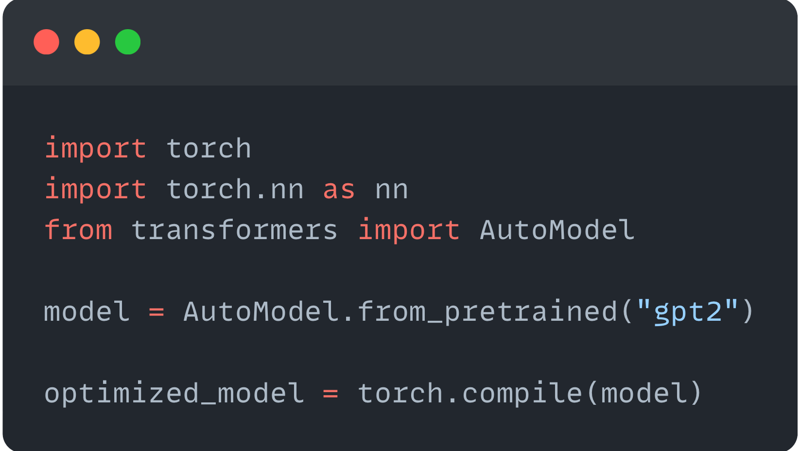
Meanwhile, FlashAttention is also being integrated into common ML frameworks, making adoption extremely simple, without the need to write a single line of CUDA C++ code. For example, FlashAttention 2 has been integrated into the PyTorch 2.2 release, which means that we can run our PyTorch models with a fused FlashAttention 2 kernel with a simple torch.compile. Here, for example, I instantiate a GPT-2 model with FlashAttention on a fused attention kernel in 5 lines of code:
To me, the most surprising aspect in the FlashAttention saga so far is how long it took the community to discover and exploit the inefficiency in the GPU’s memory access patterns in standard attention implementations. This is a good reminder that purely architectural modeling innovations are really just a small piece of the ML puzzle. In this particular case, simply looking closely what our GPUs are doing beats an entire host of modeling innovations that have been published over several years — without sacrificing predictive accuracy.
Very neat and clean explanation of flashattention for beginners